Evaluation of Merklization Design and Performance in SYCL

Created : December 31, 2021

Around a fortnight back I wrote about OpenCL accelerated Merkle Tree construction technique, while using Rescue Prime Hash as underlying collision resistant, cryptographic hash function for obtaining immediate parent node from two children nodes ( either leaves/ intermediates ). You can find that post here.

During last two weeks, I've made some improvements in Rescue Prime Hash implementation and also ported it to SYCL. If you happen to be specifically interested in those changes/ improvements, I suggest you take a look at following pull requests.

• Porting vectorized OpenCL Rescue Prime to SYCL
• Optimizing SYCL Rescue Prime with reduced vector lanes

Along with that I also explored a different way of Merklization, where given problem statement is same as before i.e. when N -many leaf nodes of some Binary Merkle Tree are provided with and (N - 1) -many intermediate nodes to be computed. In this new way of Merklization, I change which work-items are tasked to compute which intermediate nodes and how many kernel dispatch rounds are required for computing all intermediate nodes. But, as usual, that itself comes with its benefits and drawbacks. Today in this post, I plan to study design and performance of two Merklization techniques, that I've devised, while using SYCL for implementation.

Same as last post, I'm not going to be explaining how I improved Rescue Prime implementation in SYCL, but I note that a huge portion of Merklization performance boost comes from optimized implementation of Rescue Prime in SYCL. I'll do a deep study of that in coming weeks, as promised before.

Let me begin with the simple one, which henceforth I'll call Merklization approach 1. Here merklize function is provided with N -many leaf nodes, where N = 2ⁱ ∀ i ∈ {1, 2, ...}. (N - 1) -many intermediate nodes are computed by dispatching compute kernel log₂N times. Say for example, if I start with N = 32, all intermediates are computed in 5 rounds, as shown below.

You should also notice, there are 5 rounds and each of them are data dependent on previous dispatch round. But good news is that each of these rounds are easily parallelizable, due to absence of any intra-round data dependency. For some specific dispatch round if input to merklize has N intermediate/ leaf nodes, each pair of consecutive nodes are read by respective work-items ( N >> 1 in total ) which are merged into single Rescue Prime digest and stored in proper memory allocation. There is scope of global memory access coalescing, as non-strided, contiguous memory addresses are accessed by each work-item. Let us take help of a diagram to better appreciate the scope of parallelism.

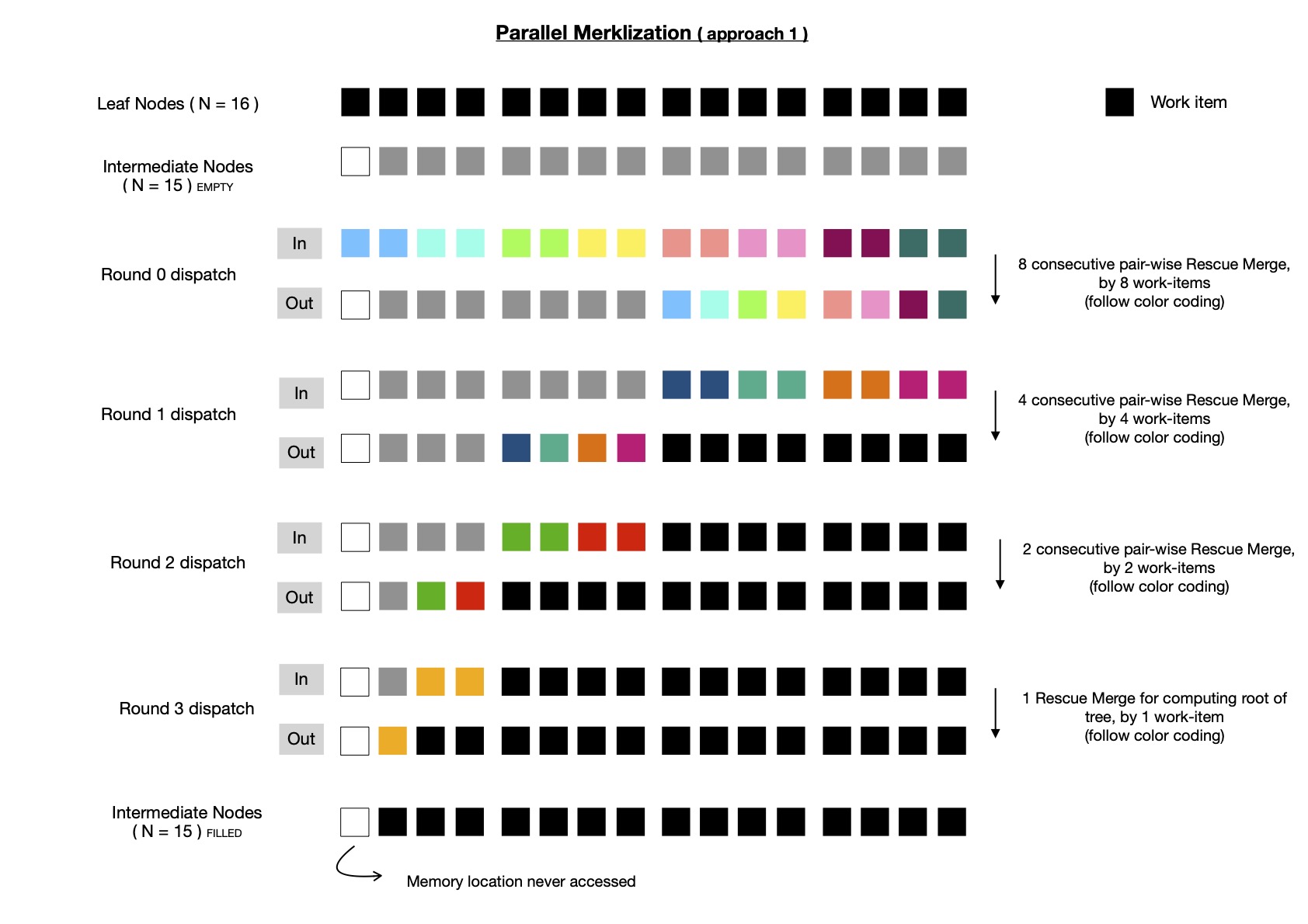
In above diagram, N ( = 16 ) -many leaf nodes are used for depicting execution flow. It requires 4 kernel dispatch rounds to compute all intermediates and each of them are data dependent on previous round. Each dispatch round shows how many work-items are required to parallelly compute all computable intermediate nodes, by invoking Rescue merge function; which work-item accesses which pair of consequtive nodes ( either leaves/ intermediates; leaves applicable only during round 0 ). Note, very first memory location ( resevered for some Rescue Prime digest ) is never accessed by any of dispatched kernels, because (N - 1) -many intermediate nodes are stored in memory allocated for storing total of N -many intermediate nodes, where N is power of 2 i.e. ( N & (N - 1) == 0 ).

Implementing this in SYCL is pretty easy, using USM allocation allows me to perform pointer arithmetics, which is much more familiar compared to SYCL buffer/ sub-buffer/ accessor. If you've gone through my last post, where I walked you through equivalent implementation using OpenCL, you should notice as SYCL 2020 USM based memory allocation is being used no such issue of device memory base address alignment is encountered here. I suspect, if I had to implement SYCL variant using SYCL buffer/ sub-buffer/ accessor abstraction ( which is useful due to its automatic dependency chain inference ability ) I could have stumbled upon alignment issues while sub-buffering. Also SYCL being single source programming model, it's much easier to program compared to raw OpenCL --- less verbosity is encountered. I suggest you take a look here for exploring exact implementation details of approach 1.

Notice when N is relatively large, say = 2²⁴, total 24 kernel dispatch rounds will be required to compute all intermediate nodes. Dispatching kernel requires host-device interaction, which is not cheap. Also OpenCL/ SYCL doesn't yet allow recording commands into a buffer and then replaying same when required to be executed as I can do in Vulkan Compute; with that during actual kernel execution, host-device interaction can be reduced and more work will be ready for offloading, while suffering less from host latencies due to say context switching. Well, OpenCL has this extension just to experiment with that idea, but today I'm working with SYCL, where I've not yet discovered anything similar. Motivated by this reason, I decided to devise a way so that kernel dispatch round count can be reduced while Merklizing.

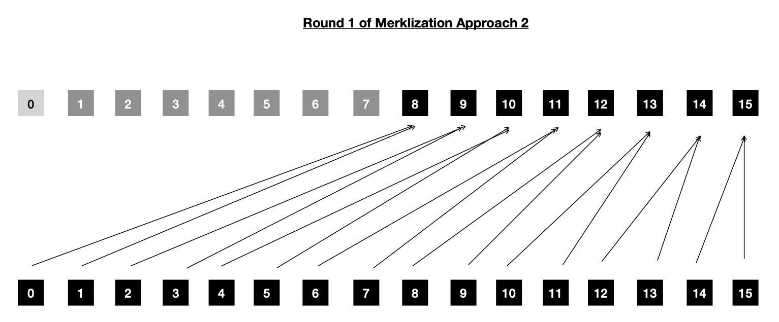
I'm going to refer to this new Merklization technique as approach 2. Say we've N = 2²⁴ -many leaf nodes and we're using work-group size B = 2⁸, then number of required kernel dispatch rounds for constructing Merkle Tree using approach 2 will be log₂(N >> (2 + log₂B)) + 1, which turns out to be 15, much lesser than 24, which would be required using approach 1. Also note, it doesn't matter what is work-group size, required #-of kernel dispatch rounds will always be log₂N using approach 1. But using approach 2, work-group size can influence total #-of required kernel dispatch rounds to compute whole Merkle Tree. If I increase work-group size B to say 2⁹, then following aforementioned formula, I'll be required to dispatch kernel 14 times. But as per my experience, increasing work-group size to that large value benefits less, which we'll explore soon. Say, finally I decide to live with work-group size B = 2⁶, I'll be required to perform 17 rounds of kernel dispatch, which is still lesser than 24 rounds, required in approach 1.

I've come up with following formula for computing required #-of kernel dispatch rounds using approach 2. You should notice, an appended + 1, in each of these cases, that's coming from here --- the very first round of kernel dispatch reads all N -many leaves from input buffer and writes (N >> 1) -many intermediate nodes ( living just above leaf nodes ) in designated location of output buffer. After that remaining intermediate nodes are computed in one/ many rounds. Note, each of these kernel dispatch rounds are data dependent on previous one, which is due to inherent hierarchical structure of Merkle Tree.

Let me now explain approach 2, while attempting to foresee what kind of (dis-)advantage it may bring to Merklization.

Say N = 16 and work-group size I'm willing to work with is 2. Then during first round, 8 work-items will be dispatched, each computing single Rescue Prime merge and total 8 intermediate nodes will be produced, who lives just above leaf nodes. Following above formula, I need to dispatch kernel 3 times for constructing whole Merkle Tree. First round looks like below.

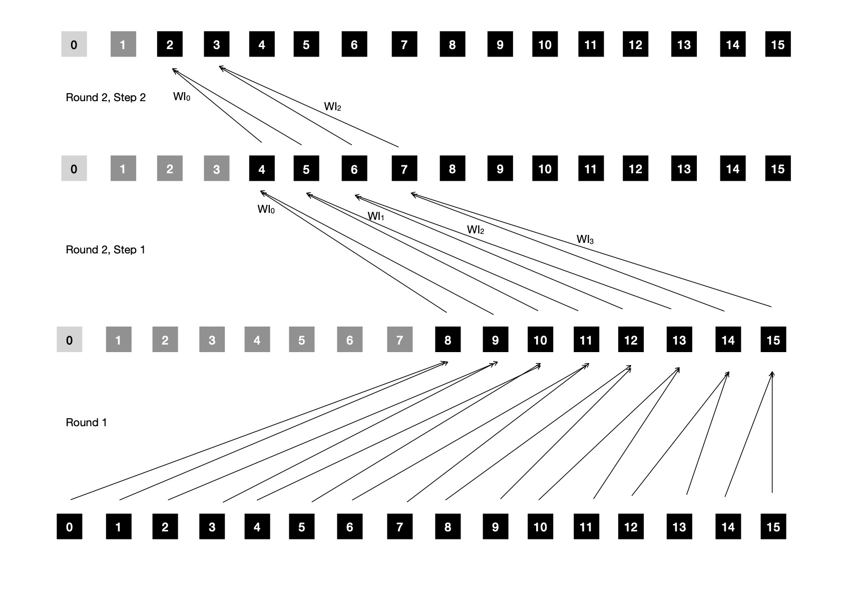
During next round, which is dependent on first one, 4 work-items will be dispatched. As first step, each of these 4 work-items will be computing one Rescue Prime merge, producing 4 intermediate nodes. These four work-items are globally numbered as {group: 0 => {0, 1, 2, 3}}, but remember I decided to work with work-group size of 2, so local indexing of 4 work-items will be {group: 0 => {0, 1}, group: 1 => {0, 1}}. After first step in round 2, all work-items present in each of work-groups are synchronized, so that it's ensured that next step can be proceeded into safely, without getting into trouble of data race. After all work-items ( = 2, in number ) in work-group reach sycl::group_barrier(...), only even indexed work-items are chosen for computing next level of intermediate nodes, which ensures odd indexed work-items don't cause any data race. After all even indexed work-items have computed upper level of intermediate nodes, all work-items in a work-group are synchronized again just to ensure that this iteration step's data will be available ( i.e. visible to next set of active work-items ) for use in next iteration. Now question is when to stop this iterative process ?

I use (1 << (iter - 1)) < B as iteration control condition, where iter = 1 at start and then iter++ after each iteration completes.

Going back to our example, where work-group size B = 2, iter = 1 should be only iteration, as after iter++ stopping criteria is reached ( 2 < 2 == !true ). Looking at following diagram also asserts so, only root of tree is left to be computed, which will be done in last kernel dispatch round.

In third and last kernel dispatch round, only 1 work-item is launched for computing root of Merkle Tree and no more iterations are required ( step two can be skipped ), because there is nothing else left for computation. Once again going back to approach 2, I'll demonstrate with N = 256 and B = 16 so that you can appreciate the need for work-group sychronization and also understand how costly it can become.

Formula says, 3 kernel dispatch rounds should be enough to compute all intermediate nodes of Binary Merkle Tree with 256 leaf nodes. In first round, 128 work-items are dispatched for computing 128 intermediate nodes, living just above 256 leaf nodes. In second kernel dispatch round, 64 work-items are dispatched for first computing 64 intermediate nodes from 128 intermediate nodes, computed during last round of dispatch. Remember B = 16 is our work-group size, so 16 work-items per work-group are synchronized before they decide to execute next step. As per loop control condition (1 << (iter - 1)) < B, it's safe to execute loop with iter = 1. That means, 8 even indexed work-items among 16 work-items in each of 4 work-groups will be activated to compute 8 intermediate nodes, producing total of 8 x 4 = 32 intermediate nodes from 64 intermediate nodes which were computed during previous step by 4 work-groups. Let us expand into 8 even indexed work-items to be activated.

It means among following 16 work-items ( per work-group; making total of 64 -many dispatched ), who all participated in first step of second round, only even indexed 8 work-items will participate in second step i.e. iteration with iter = 1.

Following 32 work-items will be active, computing 32 intermediate nodes from 64 intermediate nodes, computed during first step of second dispatch round. This is exactly the reason behind work-group synchronization after first step ( in second kernel dispatch round ), so it's ensured that all 16 work-items in work-group have computed the intermediate node it was responsible for. And only after that 8 selected work-items ( in a work-group ) can safely use previously computed 16 intermediate nodes.

After iteration with iter = 1, all 16 work-items in work-group to be synchronized, so that necessary intermediate nodes are visible to all work-items, who will be activated during next iteration i.e. iter = 2. Before we can go and execute iteration with iter = 2, we must check loop termination condition. As assert 2 < 16, execution can proceed. This time, 4 even indexed work-items ( per work-group ) among last iteration's 8 active work-items, will be activated for computing total of 4 x 4 = 16 intermediate nodes, as shown below. Once they reach end of loop, 16 work-items ( per work-group ) are synchronized, so that path of entering next round is paved well, by ensuring memory visibility.

Iteration iter = 3 can be executed, as loop termination condition doesn't yet satisfy ( i.e. assert 4 < 16 ). In this iteration, 2 even indexed work-items among last iteration's 4 active work-items ( per work-group ) will be activated for computing total 2 x 4 = 8 intermediate nodes, shown below. After completion of this iteration, all work-items in work-group will be synchronized, as usual.

Last iteration of second round i.e. iter = 4, will activate 1 ( and only one ) even-indexed work-item among 2 active work-items from last iteration ( per work-group ) and produce total of 4 intermediate nodes, which looks like below. Note this is last iteration because after that with iter = 5 loop termination condition ( i.e. (1 << (iter - 1)) < 16 ) is triggerred.

Actual reason behind stopping iteration is that I can't synchronize across work-groups, which will be required in next iteration, if I've to proceed. If I decide to go with iter = 5, I need to compute 2 intermediate nodes from (total) 4 intermediate nodes computed during last iteration. But those 4 input intermediate nodes are computed by 4 different work-items who are part of 4 different work-groups ( see above depiction ).

Question is when to start executing iteration with iter = 5 ?
Answer is when 32 work-items ( across each of two possible consecutive pair of work-groups ) agree that they've completed previous iteration & data written to global memory during that is safely available for consumption.

As it's not possible to synchronize across work-groups, I can't safely start executing next iteration i.e. iter = 5. There's a high chance that I'll end up reading intermediate node data when it's still in undefined state.

If I had a mechanism to synchronize across work-groups, following depicts which work-items will be active during iteration iter = 5.

As that is not possible, I'll have to dispatch another ( final ) round of kernel, for computing remaining intermediate nodes. Before I get to that I'd like to check how many intermediate nodes are already computed among 255 target intermediate nodes. Following table shows I've to still compute 3 intermediate nodes, which are root of Merkle Tree and their two immediate children.

In final kernel dispatch round, I'll dispatch 2 work-items ( in single work-group ), who will compute 2 intermediate nodes in step one from previous round's 4 computed intermediate nodes. After step one, these two work-items are synchronized so that in step two previous step's global memory changes ( i.e. write ops ) are ensured to be visible in correct state. In step two, first loop initiation/ termination condition is checked i.e. assert 1 < 2 and only even indexed work-item is activated to execute loop body, which computes root of Merkle Tree. With that all intermediate nodes are computed for Binary Merkle Tree with N = 256 leaf nodes.

Few points to note here, if we increase work-group size for kernel dispatches in approach 2, it seems to be beneficial because as per our formula lesser kernel dispatch rounds will be required. But approach 2 also requires us to perform work-group level synchronization, that means when work-group size is doubled up, double -many work-items will be required to synchronize so that safely next iteration can be executed, while consuming previous iteration's global memory writes ( intermediate nodes computed during last iteration/ step ). And I also note synchronization is costly. Another point to note, after every round of work-group synchronization half of previous round's active work-items ( in a work-group ) are deactivated that means most of work-items are not doing any useful work, which is just waste of computation ability of highly parallel GPU architecture.

If you happen to be interested in inspecting approach 2 in detail, I suggest you take a look at this SYCL implementation.

Now it's time to benchmark both of these implementations to actually see what do they bring on table. I used Nvidia Tesla V100 for that purpose, while compiling single source SYCL program with SYCL/ DPC++ ( experimental CUDA backend ). I'm also placing last column which shows results obtained by benchmarking equivalent OpenCL implementation of approach 1, which I already presented at end of this post.

As speculated, approach 1 is ~2x faster compared to approach 2. Though approach 2 has lesser kernel dispatch rounds but costly work-group level synchronization, mostly ( which keeps increasing after every step/ iteration ) inactive work-items etc. are reasons behind lower performance. While in approach 1, there may be log₂N -many dispatch rounds, but during each dispatch every work-item does some useful work, hence compute ability of GPU is better utilized, resulting into better performance. Equivalent OpenCL implementation of Merklization approach 1 doesn't perform as good as SYCL variant. Note, SYCL with CUDA backend uses PTX as IR, but OpenCL on Nvidia GPU uses SPIR as Intermediate Representation language. I'd like to also note, OpenCL implementation is powered by Rescue Prime merge(...) function where hash state is represented using vector with 16 lanes ( each of 64 -bit width ) i.e. ulong16. But in SYCL implementation Rescue hash state is represented using an array of 3 vectors each 4 lanes wide ( each vector lane is of 64 -bit width ) i.e. sycl::ulong4[3]. That means, in OpenCL implementation, last 4 lanes are used for padding purpose, because Rescue Prime hash state is 12 field elements ( 64 -bit each ) wide, wasting both compute and memory capability of accelerator; though it's much easier to program and more readable. I implemented Rescue Prime hash with hash state represented using both sycl::ulong16 and sycl::ulong4[3] and performance improvement I noticed in later variant is non-negligible. This improvement in Rescue merge routine indeed boosts SYCL implementation, compared to equivalent OpenCL one.

With this I'll wrap up today. You can find SYCL implementation of both merklize(...) routines here. For OpenCL variant take a peek at this repository. In coming days, I plan to talk about other topics which I'm exploring/ will explore. Have a great time !